Your first RABIES run

In this tutorial you will take two raw mouse fMRI scans and carry them all the way through the three RABIES stages: preprocess, confound_correction and analysis. Along the way you will look at the quality control images RABIES produces, so that by the end you will have seen every part of the software in action.

You do not need to understand every option you type. The point is to build a feel for the shape of a RABIES run. Everything you use here is explained elsewhere, and this page links to the relevant pages as it goes.

What you will end up with

Three output folders that mirror the three stages of the software:

rabies_tutorial/
├── bids_inputs/                  the data you download in step 2
├── preprocess_outputs/           step 3
├── confound_correction_outputs/  step 5
└── analysis_outputs/             step 6

How long this takes

Steps 1 and 2 take a few minutes. Step 3 is real image processing on real brains, and is the long one — expect it to run for an hour or more, depending on how many cores your machine has. Steps 5 and 6 take a couple of minutes each. Start step 3 and come back to it.

Step 1: Install the container

RABIES has a lot of non-Python dependencies, so you will use the prebuilt container. Install Apptainer, then build the RABIES image:

apptainer build rabies.sif docker://ghcr.io/cobralab/rabies:latest

This downloads roughly a gigabyte and takes a few minutes. When it finishes you will have a single file, rabies.sif, which contains the entire software environment.

Check that it runs:

apptainer run rabies.sif --help

You should see the RABIES usage message, listing the three processing stages: preprocess, confound_correction and analysis. That is the structure of the whole tutorial.

Tip

If you are on macOS or Windows, or Apptainer is not available to you, use Docker instead — see How to install RABIES. Every apptainer run ... -B src:dst below becomes docker run ... -v src:dst.

Step 2: Get the example data

Make a working directory and download the two-subject example dataset:

mkdir -p rabies_tutorial && cd rabies_tutorial
curl -L -o test_dataset.zip https://zenodo.org/records/8349029/files/test_dataset.zip
unzip test_dataset.zip -d bids_inputs

Look at what you got:

find bids_inputs -name '*.nii.gz'

Two subjects, each with one anatomical scan and one resting-state functional scan:

bids_inputs/
├── sub-PHG001/ses-3/
│   ├── anat/sub-PHG001_ses-3_acq-RARE_T2w.nii.gz
│   └── func/sub-PHG001_ses-3_task-rest_acq-EPI_run-1_bold.nii.gz
└── sub-PHG002/ses-3/
    ├── anat/sub-PHG002_ses-3_acq-RARE_T2w.nii.gz
    └── func/sub-PHG002_ses-3_task-rest_acq-EPI_run-1_bold.nii.gz

Notice the file names. The sub-, ses-, task- and T2w/bold parts are not decoration — this is the BIDS naming standard, and it is how RABIES finds the scans and pairs each functional image with the anatomical image from the same session. Your own data will need to look like this too. See Input data requirements.

Step 3: Preprocess

Create the output folder, then run the preprocessing stage:

mkdir -p preprocess_outputs

apptainer run \
  -B $PWD/bids_inputs:/inputs:ro \
  -B $PWD/preprocess_outputs:/outputs \
  rabies.sif -p MultiProc \
  preprocess /inputs /outputs \
  --anatomical_resampling 0.15x0.15x0.15 \
  --anat_inho_cor multiotsu=true

Breakdown of the command:

-B $PWD/bids_inputs:/inputs:ro makes your input folder visible inside the container under the name /inputs, read-only. The container cannot see any path you do not bind, which is why the RABIES arguments say /inputs and /outputs rather than the paths on your machine.
-p MultiProc runs the pipeline in parallel across the cores of your machine. Leave it out and everything runs one step at a time.
--anatomical_resampling 0.15x0.15x0.15 commands to resample the images to 0.15mm isotropic resolution for each registration operation. This resolution is a decent heuristic in practice for a mouse brain to derive ‘good-enough’ alignment for standard EPI images while speeding things up for high resolution structural images. We do not recommend registration in non-isotropic resolution.
--anat_inho_cor multiotsu=true activates the multiotsu option for inhomogeneity correction of anatomical images, which carries a more aggressive correction (for most datasets this is not necessary, you should not use this by default, here it’s because this particular dataset has an especially sharp intensity gradient).

You did not specify an atlas. The container comes with the DSURQE mouse atlas already installed, and RABIES uses it by default (see built-in template files).

Let it run. You will see a stream of Nipype log lines as each node in the workflow completes.

Step 4: Look at the registration quality control report

This is a crucial step in practice — this is where you’ll catch alignment issues that can completely break later stages. Open the report folder:

ls preprocess_outputs/preprocess_QC_report/

Each subfolder holds PNG images for one key preprocessing step that requires visual quality control (formally documented here). You will go through each subfolder in order, as later steps depend on the success of the first ones.

First open preprocess_outputs/preprocess_QC_report/anat_inho_cor which displays the inhomogeneity correction step for the structural scans.

Four-column figure showing the stages of structural inhomogeneity correction — Fig. 1 Four panels of the inhomogeneity correction report, representing the initial and final iterations of inhomogeneity before/after brain masking.

Your outputs should resemble the above example, where brain masking was successfully delineating the brain edges, and the prominent intensity gradient in the image is properly corrected for (partly thanks to the multiotsu=true option we selected above).

The success of this inhomogeneity correction is crucial for the registration step below, as errors here can leave intensity biases that do not match across images, or even cropped out brains from masking errors.

Then, you can consult the alignment of each image to the dataset average (of only 2 scans in this case) within preprocess_QC_report/commonspace_reg_wf.Anat2Unbiased/.

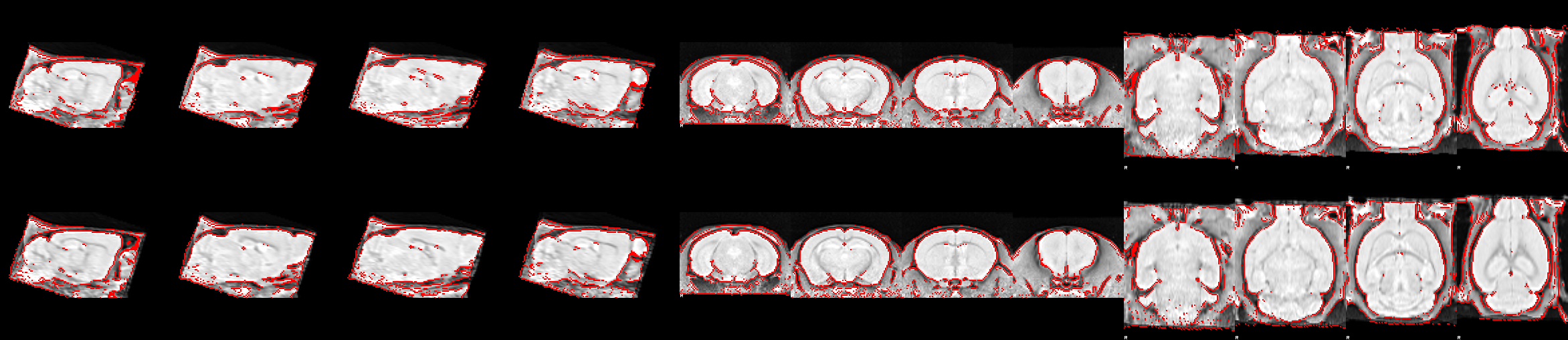
Overlap to the study template — Fig. 2 The alignment of your data (top) with the study template (bottom). The outlines should follow the same anatomy.

The alignment here determines whether an entire scanning session is properly aligned to common space. An error here will result in bad anatomical masks that impact EPI preprocessing steps below, and ultimately misaligned timeseries at the end of preprocessing.

Next, you should validate the registration of the study template to the external commonspace template in preprocess_QC_report/commonspace_reg_wf.Unbiased2Atlas/.

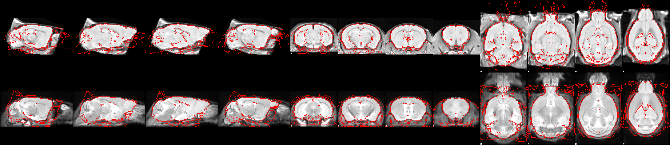
Overlap of the study template on the reference atlas — Fig. 3 The alignment of your study template (top) with the external commonspace template (bottom). The outlines should follow the same anatomy.

The alignment to the external atlas is the last step that can link up the set of brain masks that are then used for inhomogeneity correction/registration of the EPI below, and also regulates the eventual resampling of timeseries to common space.

We then move on to the EPI preprocessing steps. You can open the preprocess_QC_report/bold_inho_cor/ folder, where you will validate the inhomogeneity correction of each EPI scan.

Four-column figure showing the stages of functional inhomogeneity correction — Fig. 4 Same four panels of the inhomogeneity correction report as with the structural scan, but now for the EPI scan.

Again here you should find adequate brain masking and intensity correction. An error here would impact the EPI registration below.

Finally, open preprocess_QC_report/EPI2Anat/, which shows each functional scan aligned onto its own anatomical scan:

Overlap of a functional scan on its anatomical scan — Fig. 5 The functional image (top) matched to the anatomical image (bottom) from the same session. This registration is also what corrects susceptibility distortion.

It is unlikely that this registration step will work if any of the previous steps failed significantly for a given run/session.

On this example dataset, each preprocessing step should run without error. When they do not on your own data, How to troubleshoot registration will help you fix it.

Step 5: Correct confounds

Preprocessed data is not yet ready to analyse: the next stage is critical for removing head motion and physiological artefacts that produce correlations that corrupt functional connectivity.

mkdir -p confound_correction_outputs

apptainer run \
  -B $PWD/bids_inputs:/inputs:ro \
  -B $PWD/preprocess_outputs:/outputs \
  -B $PWD/confound_correction_outputs:/cc_outputs \
  rabies.sif -p MultiProc \
  confound_correction /outputs /cc_outputs \
  --frame_censoring FD_censoring=true,FD_threshold=0.05 \
  --nuisance_regressors mot_6 aCompCor_5 \
  --smoothing_filter 0.3

Note that you bind bids_inputs again even though it is not in the RABIES arguments. Each stage reads the file paths recorded by the previous one, so every path used in step 3 has to stay reachable, at the same location, for the rest of the pipeline.

The options you passed:

--frame_censoring FD_censoring=true,FD_threshold=0.05 applies censoring of high-motion frames using a 0.05 mm threshold on framewise displacement.
--nuisance_regressors mot_6 aCompCor_5 models the signal using the six head motion parameters plus the first 5 aCompCor principal components derived from the combined WM-CSF masks, and subtracts the variance explained by those regressors.
--smoothing_filter 0.3 applies 0.3 mm Gaussian spatial smoothing.

That is a relatively modest correction. Choosing a correction strategy for a real dataset is its own task, covered in How to optimise your confound correction strategy.

The cleaned timeseries land in confound_correction_outputs/confound_correction_datasink/cleaned_timeseries/.

Step 6: Analyse

Now compute seed-based connectivity using a pre-built seed, and generate data quality reports using --data_diagnosis:

mkdir -p analysis_outputs

apptainer run \
  -B $PWD/bids_inputs:/inputs:ro \
  -B $PWD/preprocess_outputs:/outputs \
  -B $PWD/confound_correction_outputs:/cc_outputs \
  -B $PWD/analysis_outputs:/analysis_outputs \
  rabies.sif -p MultiProc \
  analysis /cc_outputs /analysis_outputs \
  --data_diagnosis \
  --seed_list SS_frontal_seed 

Breakdown of the command:

--seed_list SS_frontal_seed will use the pre-built seed in the frontal cortex for deriving seed-based connectivity in each scan.
--data_diagnosis will generate a set of data quality reports associated to the functional connectivity analysis results.

You have now carried out a basic functional connectivity analysis, and generated the scan-level spatiotemporal diagnosis report for each scan, which you can now open from analysis_outputs/data_diagnosis_datasink/figure_temporal_diagnosis/ and analysis_outputs/data_diagnosis_datasink/figure_spatial_diagnosis/ subfolders. This report is part of a larger data quality assessment framework developed for rodent fMRI along with RABIES. Some group-level reports were not generated here, as those require at minimum 3 scans. It takes time to learn how to read these reports, and some experience to interpret them accurately. For the sake of the tutorial, we will simply validate whether we can observe a brain network from seed-based connectivity. Let’s open the spatial diagnosis report under analysis_outputs/data_diagnosis_datasink/figure_spatial_diagnosis/:

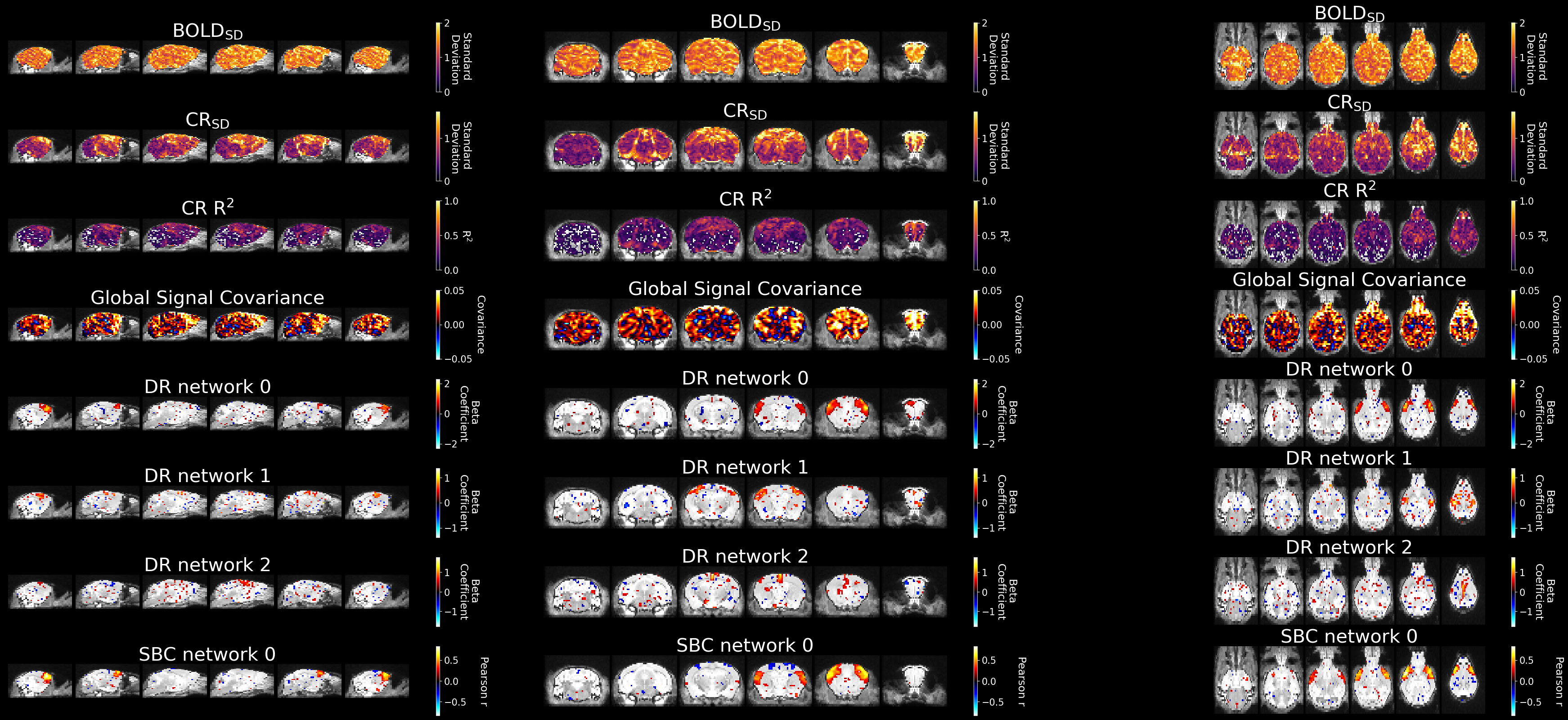
Tutorial spatial diagnosis report — Fig. 6 Spatial diagnosis report for the first subject.

In this report, the resulting seed-based connectivity can be visualised in the last row labelled ‘SBC network 0’. We can see in those two example scans that the seed revealed a bilateral correlation structure that corresponds to the somatomotor network anatomy of the mouse brain. This confirms that this network was adequately mapped and measured (although more subtle confounding effects could still exist, but that is a question beyond the scope of the tutorial).

These connectivity maps are saved and can be accessed as NIfTI files in the analysis_outputs/commonspace_analysis_datasink/seed_correlation_maps output folder, and could be fed into downstream statistical analyses in an actual experiment.

What you have done

You have run all three RABIES stages and produced a connectivity estimate from raw scans. Specifically, you:

built the container and confirmed it runs
preprocessed two subjects, registering them into a common atlas space
inspected the registration quality control images
removed motion and physiological confounds from the timeseries
computed a seed-based connectivity on each scan
confirmed the mapping of the somatomotor network using the scan-level diagnostic report

Where to go next

For your own data, the decisions the tutorial made for you become yours to make:

Your data has to be in BIDS format — see Input data requirements.
Your registrations will not always succeed on the first try — see How to troubleshoot registration.
Confound correction should be tuned to your data, not copied from a tutorial — see How to optimise your confound correction strategy and How to assess data quality.
To understand what the preprocessing actually did, read The preprocessing workflow.