The confound correction workflow

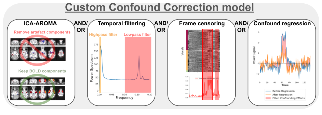
Diagram of the RABIES confound correction workflow — Fig. 17 The confound correction workflow.

The confound correction workflow brings together a broad set of standard tools from the human literature. Each step’s implementation follows best practices and is structured to prevent the re-introduction of confounds, as recommended in [PML+14] and [LGWC19].

Every operation is optional (at minimum the temporal mean is removed), and a set of operations can be selected to design a customised workflow.

Important

There is no universally optimal correction strategy. We provide guidelines for tuning the pipeline to address quality issues you can actually identify in your data — see Data quality assessment and How to optimise your confound correction strategy.

1. Frame censoring

--frame_censoring

Frame censoring temporal masks are derived from FD and/or DVARS thresholds and applied to the BOLD timeseries first, before any other correction step, to exclude signal spikes which would otherwise bias detrending, frequency filtering and confound regression [PML+14].

Censoring with framewise displacement: Applies frame censoring based on a framewise displacement threshold. Frames exceeding the threshold, together with 1 frame back and 2 frames forward, are masked out [PBS+12].
Censoring with DVARS: The DVARS values are z-scored (\(DVARS_Z = \frac{DVARS-\mu}{\sigma}\), where \(\mu\) is the mean DVARS across time and \(\sigma\) the standard deviation), and frames with \(|DVARS_Z|>2.5\) are removed. Z-scoring and outlier detection are repeated within the remaining frames, iteratively, until no further outlier is detected.
--match_number_timepoints: Constrains every scan to retain the same final number of frames, to avoid downstream effects of unequal temporal degrees of freedom (tDOF) on analysis. A pre-set final number of frames is defined with minimum_timepoint, and the surplus frames remaining after censoring — accounting for the edge removal in step 4 — are selected at random and removed.

2. Detrending

--detrending

Detrending is applied at the inputted polynomial order (e.g. 0 only removes the intercept, 1 for linear, 2 for quadratic, etc.). Detrended timeseries \(\hat{Y}\) are obtained by ordinary least squares (OLS) linear regression:

\[ \beta = OLS(X,Y) \]

\[ \hat{Y} = Y - X\beta \]

where \(Y\) is the timeseries and the regressors are the polynomial expansions of the time axis, e.g. \(X = [intercept, time, time^2]\) for --detrending order=2.

3. ICA-AROMA

--ica_aroma

Cleaning of motion-related sources using the ICA-AROMA [PMvR+15] classifier. The hard-coded human priors for anatomical masking and the linear coefficients for classification were adapted from the original code to function with rodent images.

ICA-AROMA is applied before frequency filtering, to remove effects of motion that would otherwise produce ringing after filtering [Car13, PMvR+15].

4. Frequency filtering

--TR / --highpass / --lowpass / --edge_cutoff

Spectral interpolation of censored timepoints: Frequency filtering needs special handling after frame censoring, because conventional filters cannot handle missing data. RABIES implements the method of [PML+14], which interpolates the data while preserving its frequency composition. It relies on an adaptation of the Lomb-Scargle periodogram, which estimates the frequency composition of the timeseries despite missing data points; from that estimate, missing timepoints are simulated with the frequency profile preserved [MGG+04].
Butterworth filter: Following the simulation, highpass and/or lowpass filtering is applied using a 3rd-order Butterworth filter (scipy.signal.butter). After filtering, the temporal mask from censoring is re-applied to remove the interpolated timepoints.

Tip

Edge artefacts are introduced by standard frequency filters: for a highpass at 0.01Hz, we recommend removing 30 seconds at each end of the timeseries with --edge_cutoff [PML+14].

5. Nuisance regression

--nuisance_regressors

For each voxel timeseries, a selected set of nuisance regressors is modelled using OLS linear regression and their modelled contribution to the signal is removed. Prior to carrying out the linear regression, a critical implementation strategy in RABIES is to apply the same censoring, detrending and frequency filtering carried in steps 1, 2 and 4 onto the regressors themselves to mitigate the re-introduction of previously corrected confounds, as recommended in [PML+14] and [LGWC19]. After doing so, the regressed timeseries \(\hat{Y}\) are obtained with

\[\beta = OLS(X,Y)\]

\[ Y_{CR} = X\beta \]

\[ \hat{Y} = Y - Y_{CR} \]

where \(Y\) is the timeseries, \(X\) is the set of nuisance timecourses (censored, detrended and filtered), and \(Y_{CR}\) is the confound timeseries predicted from the model at each voxel — a time-by-voxel 2D matrix.

6. Intensity scaling

--image_scaling

Voxel intensity values should be scaled to improve comparability between scans and datasets. The available options:

Grand mean: Default. Timeseries are divided by the mean intensity across the brain, then multiplied by 100 to obtain percent BOLD deviations from the mean. The mean intensity of each voxel is derived from the \(\beta\) coefficient of the intercept computed during Detrending.
Voxelwise mean: As grand mean, but each voxel is independently scaled by its own intercept from detrending.
Global standard deviation: Timeseries are divided by the total standard deviation across all voxel timeseries.
Voxelwise standardization: Each voxel is divided by its own standard deviation to derive z-scored timeseries (i.e. 0-mean and unit standard deviation).
Homogenize variance voxelwise: With --scale_variance_voxelwise, and only if no voxelwise scaling was already applied, timeseries are first scaled voxelwise by their standard deviation — yielding a homogeneous variance distribution across voxels — and then re-scaled to preserve the original total standard deviation of the entire 4D timeseries, so the global standard deviation does not change. Inhomogeneous variability distribution can be a confound signature, so this option may downscale its impact. It can be combined with grand mean scaling.

7. Smoothing

--smoothing_filter

Timeseries are spatially smoothed using a Gaussian smoothing filter (nilearn.image.smooth_img).