The spatiotemporal diagnosis

The spatiotemporal diagnosis is a visual report generated for each scan independently, after dual regression or seed-based connectivity analysis. It displays a large set of temporal and spatial features for that scan, supporting assessment of potential data quality issues and of whether network connectivity has been affected.

It is generated by --data_diagnosis at the analysis stage, into data_diagnosis_datasink/figure_temporal_diagnosis/ and data_diagnosis_datasink/figure_spatial_diagnosis/.

Note

Unless stated otherwise, all metrics are computed from fMRI timeseries after the confound correction stage.

An example report

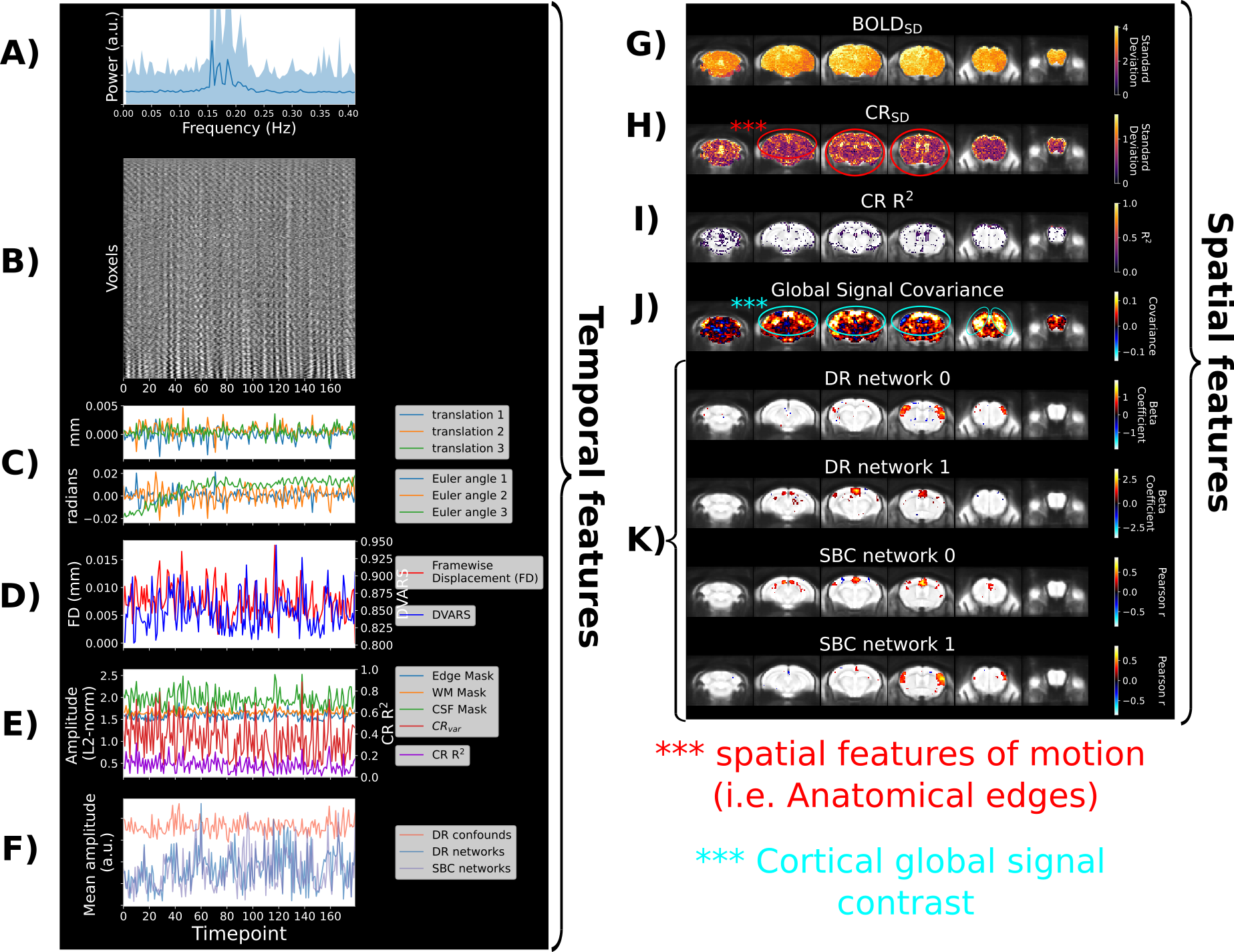
The spatiotemporal diagnosis report for a scan with clear network connectivity — Fig. 19 A scan with little confound signature and clear network connectivity. Each spatial map is shown along 6 cortical slices, overlapped onto the anatomical template in common space.

In this example both dual regression and seed-based connectivity were conducted: DR network 0 and SBC network 1 correspond to analysis of the somatomotor network, while DR network 1 and SBC network 0 correspond to the default mode network. Network maps from dual regression (DR) or seed-based connectivity (SBC) are thresholded to include the top X% of voxels with the highest values, X% being defined by --brainmap_percent_threshold.

The features are detailed below. For the exact computation behind each one, see Metric definitions.

Temporal features, top to bottom

Power spectrum: The frequency power spectrum, showing the dominant frequency profile. Always shown averaged across the whole brain; spectra for individual seeds can be added with --plot_seed_frequencies.
Carpet plot: The entire fMRI timeseries as a time-by-voxel 2D matrix. This makes global fluctuations in signal intensity visible, which is a proxy for various global artefacts [PPLM17]. Censored frames are labelled in red.
Translation and rotation head motion parameters: The 6 rigid body parameters estimated during preprocessing, tracking head position across the scan duration.
Framewise distance from the mean image: The mean square error between each frame and the average EPI, computed as the tri-mean across time voxelwise, and computed prior to confound correction to map changes in brain contrast over time. This complements framewise displacement, since it captures changes in raw image contrast across time that remain after head motion realignment and might not be well captured by framewise displacement. The metric is also output by --hmc_qc_report at the preprocess stage, and can be used for censoring via --frame_censoring at the confound_correction stage.
Framewise displacement and DVARS [PBS+12]: Framewise displacement quantifies movement between consecutive frames, revealing the timing and amplitude of spontaneous motion. DVARS — the root-mean-square of the timeseries’ temporal derivative — reveals shifts in global fMRI signal intensity, which can also indicate suspicious spikes in signal.
Variance captured and removed by confound regression: The linear model fitted during nuisance regression provides an estimate of the nuisance timeseries, from which the variance removed at each frame can be quantified. The report displays the absolute variance, as the RMS of the nuisance timeseries across voxels for each frame, and the relative variance removed, as the \(R^2\) at each frame. Together these visualise confound effects and show whether confound regression appropriately modelled the confounds detected in the other temporal features.
Mean signals within anatomical masks: The mean timecourse within the whole-brain, edge, white matter and CSF masks. The edge, WM and CSF regions are susceptible to motion and physiological confounds [PMvR+15], and contrasting them with the whole-brain global signal helps assess artefactual effects across the brain.
Mean amplitude of network vs confound timecourses: The averaged timecourses for network analyses and for confound sources are compared, to assess whether network amplitude is spurious — that is, correlated with the confound timecourse. Confound timecourses are modelled by running dual regression with a complete set of ICA components representing a mixture of networks and confounds of various origins, and compiling the timecourses from the confound components. RABIES uses this set of ICA components for mice by default.

Spatial features, top to bottom

Spatial distribution in signal variability (BOLD_SD): The signal variability, i.e. standard deviation, at each voxel. This map indexes whether significant confounds are contributing to the signal. Without influence from confounds, as in the example above, signal variability is largely homogeneous.
Confound regression variance explained (CR_SD): The variance explained by confound regression at each voxel, taken as the standard deviation of the modelled confound timecourse. This contrasts the amplitude of confound effects spatially, and can specifically delineate the presence of confounds and identify their type. In the example, minor motion signatures are identified.
Confound regression variance explained proportion: As CR_SD, but showing the proportion of variance explained (\(R^2\)).
Global signal covariance: The covariance of each voxel with the global signal. The contrast in this map reveals the predominant source of global signal fluctuation, which takes various forms depending on the contributions from neural networks and from confounds. In the ideal case there is predominant contrast in grey matter, with a shape reminiscent of a brain network, as in the example above.
Network spatial maps: The spatial network maps fitted using dual regression, or seed-based analysis, for the selected networks of interest — in the example, the somatomotor and default mode networks. These fits give insight into the quality of the network analysis and how it may affect downstream statistics.

Note

\(CR_{SD}\) and \(CR_{R^2}\) are computed from the regressors specified with --nuisance_regressors during confound correction. If no regressors are specified, they are still estimated using regression on the 6 motion parameters — but that regression is not applied to remove signal from the timeseries.

Four categories of quality outcome

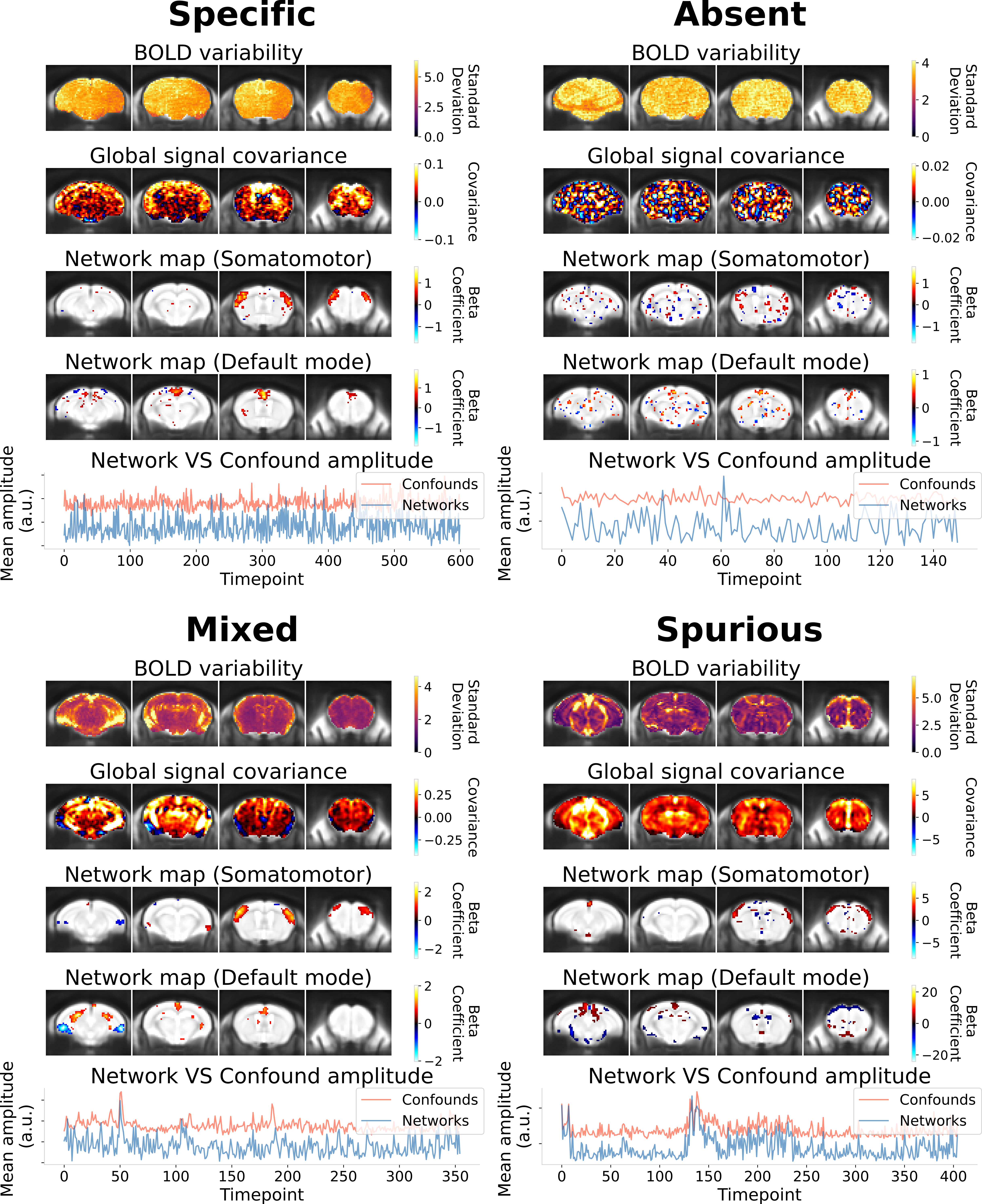
Fig. 20 Five key diagnostic features enable identifying four categories of scan quality.

A subset of the features above are the most decisive in determining scan quality in relation to connectivity analysis. We exemplify here how these can distinguish between 4 main categories of scan quality.

BOLD variability: Presents a homogeneous contrast in uncorrupted scans, and otherwise reveals the anatomical signature of a confound — this can allow recognising the type of confound present.
Global signal covariance: Sensitive to both non-neural confounds (the spurious category) and network signatures (the specific category). It therefore reflects whether network or confound sources dominate coordinated fluctuations, and delineates the most likely contributors to downstream connectivity measures.
Network map: By visualising the network maps, we can directly intuit whether they reproduce expected anatomical features of the network of interest. This is what establishes that the network is not absent (the absent category), and that its shape is not distorted by spurious features (the spurious category).
Network and confound timecourses: The respective timecourses reveal relationships between network amplitude and confounds in the temporal domain. This does not describe the type of confound, but a strong correlation in the temporal domain is the most conclusive indicator of spurious connectivity, and an important complement to inspecting network shape — spurious effects can affect amplitude while leaving shape largely intact.

These 4 features are sufficient to capture the essential characteristics of network detectability and spurious connectivity at the single scan level. The remaining features provide additional detail about timeseries properties, motion parameters and confound regression, and further support characterising the specific origin of a confound — for example, establishing that a correlation between network and confound timecourses originates from framewise displacement, i.e. from motion.